MMCCI Melanoma CCI Integration and Analysis Example

In this example, we have melanoma samples from four different technologies - Visium, CosMx, Xenium and CODEX. Each sample has been run through stLearn CCI and the outputs have been converted to CCIData objects, except for the CODEX data.

We will integrate the samples together, and then run analysis on the integrated results.

Integration

These CCI results will be integrated together in this notebook with the following steps:

1. Load the stLearn outputs and convert to be used with MMCCI

2. Integrate within platforms (Visium, CosMx, Xenium) and (Xenium + CODEX)

3. Integrate within each patient (4 different patients)

import mmcci

1. Load CCIData objects

This data is available on the GitHub repo and is created from stLearn, except for the CODEX samples which are from squidpy.gr.interaction_matrix.

Information on loading in CCI results from different tools is available here

data_dir = '../../../data/melanoma/'

visium_samples = [
    mmcci.io.read_CCIData(data_dir + 'visium1.json'),
    mmcci.io.read_CCIData(data_dir + 'visium2.json'),
    mmcci.io.read_CCIData(data_dir + 'visium3.json'),
    mmcci.io.read_CCIData(data_dir + 'visium4.json'),
    ]

xenium_samples = [
    mmcci.io.read_CCIData(data_dir + 'xenium1.json'),
    mmcci.io.read_CCIData(data_dir + 'xenium2.json'),
    mmcci.io.read_CCIData(data_dir + 'xenium3.json'),
    mmcci.io.read_CCIData(data_dir + 'xenium4.json'),
    mmcci.io.read_CCIData(data_dir + 'xenium5.json'),
    mmcci.io.read_CCIData(data_dir + 'xenium6.json'),
    ]

cosmx_samples = [
    mmcci.io.read_CCIData(data_dir + 'cosmx1.json'),
    mmcci.io.read_CCIData(data_dir + 'cosmx2.json'),
    mmcci.io.read_CCIData(data_dir + 'cosmx3.json'),
    mmcci.io.read_CCIData(data_dir + 'cosmx4.json'),
    mmcci.io.read_CCIData(data_dir + 'cosmx5.json'),
    mmcci.io.read_CCIData(data_dir + 'cosmx6.json'),
    mmcci.io.read_CCIData(data_dir + 'cosmx7.json'),
    mmcci.io.read_CCIData(data_dir + 'cosmx8.json'),
    ]

codex_samples = [
    mmcci.io.read_network(data_dir + 'codex1.csv'),
    mmcci.io.read_network(data_dir + 'codex2.csv'),
    mmcci.io.read_network(data_dir + 'codex3.csv'),
    mmcci.io.read_network(data_dir + 'codex4.csv'),
]

# These colours will be used for plotting later

colors = {
    'Endothelial': '#1f77b4',
    'Fibroblast': '#aec7e8',
    'KC Differentiating': '#ff7f0e',
    'KC Cycling': '#ffbb78',
    'KC Basal': '#2ca02c',
    'KC Other': '#98df8a',
    'NK + T': '#d62728',
    'B + PDC': '#ff9896',
    'Melanocyte': '#9467bd',
    'Myeloid': '#c5b0d5',
    'Pilosebaceous': '#8c564b',
    'NotDet': '#c49c94'
    }

Some of the celltype names are slightly different between platforms, so we can fix that with this function

cell_type_replacements = {
    'KC.Basal': 'KC Basal',
    'KC_Basal': 'KC Basal',
    'KC.Cycling': 'KC Cycling',
    'KC_Cyc': 'KC Cycling',
    'KC_Diff': 'KC Differentiating',
    'KC_Other': 'KC Other',
    'NK.T': 'NK + T',
    'B.PDC': 'B + PDC',
    'B...PDC': 'B + PDC',
}

visium_samples = [sample.rename_cell_types(cell_type_replacements) for sample in visium_samples]
cosmx_samples = [sample.rename_cell_types(cell_type_replacements) for sample in cosmx_samples]

1. Integrate within platforms

This step first normalises the samples based on the number of spots, then it integrates the CCI results together

for i in range(len(visium_samples)):
    visium_samples[i] = visium_samples[i].scale_by_nspots()
    visium_samples[i] = visium_samples[i].filter_by_p_vals(assay='scaled')
    visium_samples[i] = visium_samples[i].calc_overall(assay='filtered')
    
for i in range(len(xenium_samples)):
    xenium_samples[i] = xenium_samples[i].scale_by_nspots()
    xenium_samples[i] = xenium_samples[i].filter_by_p_vals(assay='scaled')
    xenium_samples[i] = xenium_samples[i].calc_overall(assay='filtered')
    
for i in range(len(cosmx_samples)):
    cosmx_samples[i] = cosmx_samples[i].scale_by_nspots()
    cosmx_samples[i] = cosmx_samples[i].filter_by_p_vals(assay='scaled')
    cosmx_samples[i] = cosmx_samples[i].calc_overall(assay='filtered')
    
visium = mmcci.it.lr_integration(visium_samples, method='>=50%', assay='scaled', metadata={'platform': 'visium'})
xenium = mmcci.it.lr_integration(xenium_samples, method='>=50%', assay='scaled', metadata={'platform': 'xenium'})
cosmx = mmcci.it.lr_integration(cosmx_samples, method='>=50%', assay='scaled', metadata={'platform': 'cosmx'})

# Single network integration is done differently (p_values are not used)
codex = mmcci.it.integrate_networks(codex_samples)

Integrating LR CCI scores: 100%|██████████| 1100/1100 [00:05<00:00, 208.91it/s]
Integrating p values: 100%|██████████| 1425/1425 [00:27<00:00, 51.63it/s]
Integrating LR CCI scores: 100%|██████████| 13/13 [00:00<00:00, 110.33it/s]
Integrating p values: 100%|██████████| 13/13 [00:00<00:00, 45.35it/s]
Integrating LR CCI scores: 100%|██████████| 517/517 [00:06<00:00, 79.94it/s]
Integrating p values: 100%|██████████| 517/517 [00:15<00:00, 34.03it/s]

visium = visium.filter_by_p_vals().calc_overall(assay='filtered')
xenium = xenium.filter_by_p_vals().calc_overall(assay='filtered')
cosmx = cosmx.filter_by_p_vals().calc_overall(assay='filtered')

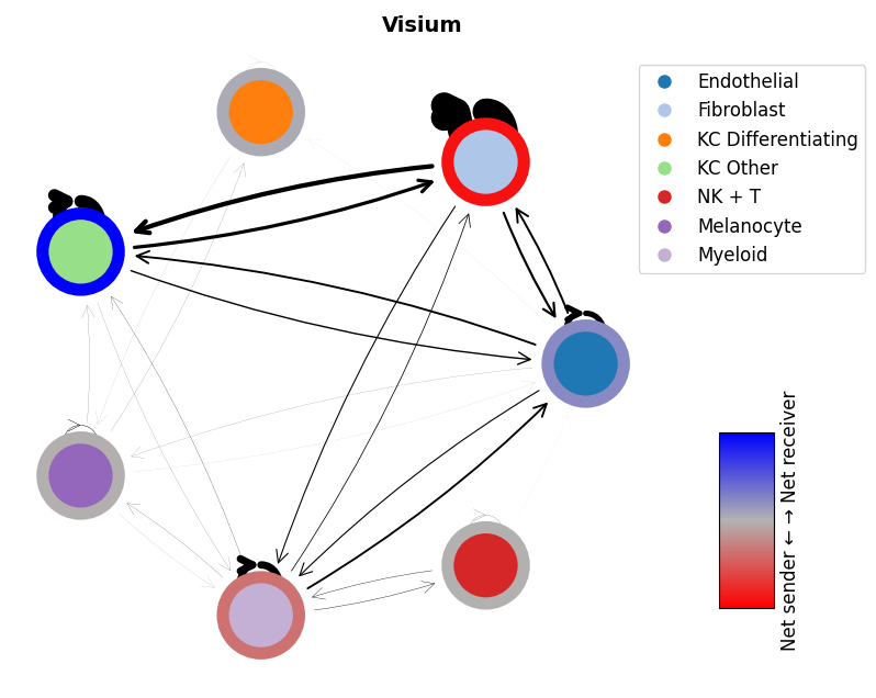
mmcci.pl.network_plot(visium.assays['filtered']['overall'], node_colors=colors, title='Visium')
mmcci.pl.network_plot(xenium.assays['filtered']['overall'], node_colors=colors, title='Xenium')
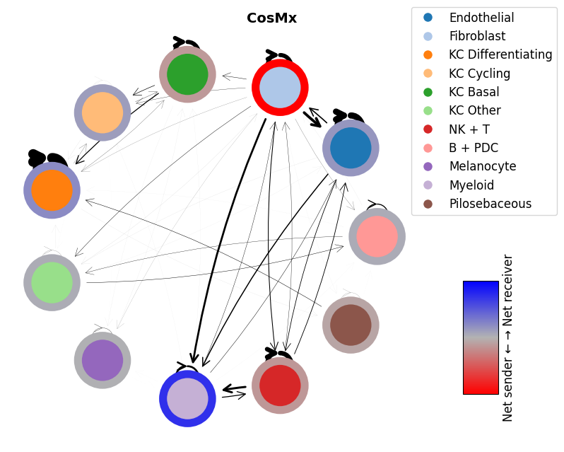
mmcci.pl.network_plot(cosmx.assays['filtered']['overall'], node_colors=colors, title='CosMx')
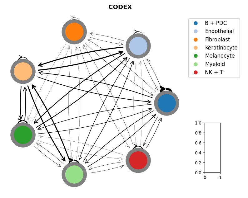
mmcci.pl.network_plot(codex.assays['raw']['network'], title='CODEX')

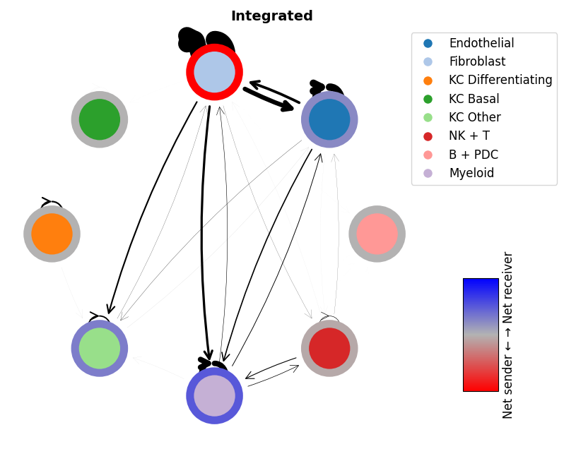
Finally, we can integrate each of these together to get a complete integrated network

scale_factors = mmcci.it.calc_scale_factors([visium, xenium, cosmx])

visium = visium.scale(scale_factors['visium'])
xenium = xenium.scale(scale_factors['xenium'])
cosmx = cosmx.scale(scale_factors['cosmx'])

integrated = mmcci.it.lr_integration([visium, xenium, cosmx], method='>=50%')
integrated = integrated.filter_by_p_vals().calc_overall(assay='filtered')

mmcci.pl.network_plot(integrated.assays['filtered']['overall'], node_colors=colors, title='Integrated')

Integrating LR CCI scores: 100%|██████████| 321/321 [00:00<00:00, 1172.02it/s]
Integrating p values: 100%|██████████| 1540/1540 [00:29<00:00, 51.60it/s]

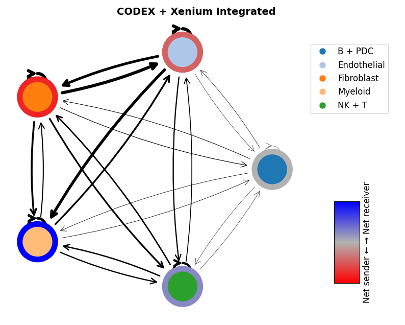
We can also integrate CODEX with other overall networks, for example Xenium

# The cell types are different between the platforms
print("Xenium cell types: ", xenium.get_cell_types())
print("CODEX cell types: ", codex.get_cell_types())

# We can join some of the cell types in the Xenium together
xenium_alt = xenium.merge_cell_types(['KC Basal', 'KC Cycling', 'KC Differentiating', 'KC Other', 'Pilosebaceous'], 'Keratinocyte')

# Now we can integrate the Xenium and CODEX overall networks
codex_xenium_integrated = mmcci.it.integrate_networks([codex, xenium_alt], assay=['raw', 'filtered'], network_key=['network', 'overall'])

mmcci.pl.network_plot(codex_xenium_integrated.assays['raw']['network'], title='CODEX + Xenium Integrated')

Xenium cell types:  ['KC Basal', 'NK + T', 'KC Cycling', 'Pilosebaceous', 'Fibroblast', 'Endothelial', 'B + PDC', 'KC Differentiating', 'Myeloid', 'Melanocyte', 'KC Other']
CODEX cell types:  ['NK + T', 'Fibroblast', 'Endothelial', 'B + PDC', 'Myeloid', 'Keratinocyte', 'Melanocyte']

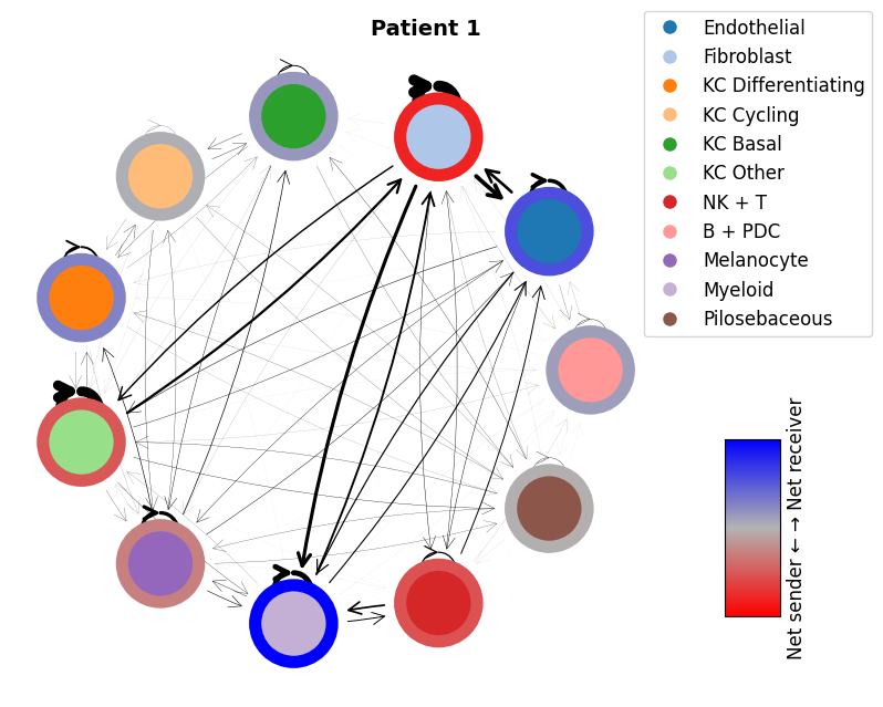
3. Integrate by patient

We use the same normalised CCI results as before but integrate by patient now

# Define the samples that each patient has

patient_1 = [visium_samples[3], cosmx_samples[0]]
patient_2 = [visium_samples[1], cosmx_samples[1], cosmx_samples[2]]
patient_3 = [visium_samples[0], cosmx_samples[3], cosmx_samples[4], cosmx_samples[5]]
patient_4 = [visium_samples[2], cosmx_samples[6], cosmx_samples[7]]

patient_1_integrated = mmcci.it.lr_integration(patient_1, method='>=50%', assay='scaled')
patient_2_integrated = mmcci.it.lr_integration(patient_2, method='>=50%', assay='scaled')
patient_3_integrated = mmcci.it.lr_integration(patient_3, method='>=50%', assay='scaled')
patient_4_integrated = mmcci.it.lr_integration(patient_4, method='>=50%', assay='scaled')

Integrating LR CCI scores: 100%|██████████| 1037/1037 [00:00<00:00, 7334.44it/s]
Integrating p values: 100%|██████████| 1037/1037 [00:20<00:00, 49.60it/s]
Integrating LR CCI scores: 100%|██████████| 516/516 [00:04<00:00, 111.21it/s]
Integrating p values: 100%|██████████| 1326/1326 [00:26<00:00, 50.10it/s]
Integrating LR CCI scores: 100%|██████████| 510/510 [00:06<00:00, 79.19it/s]
Integrating p values: 100%|██████████| 1489/1489 [00:28<00:00, 51.69it/s]
Integrating LR CCI scores: 100%|██████████| 517/517 [00:00<00:00, 1051.82it/s]
Integrating p values: 100%|██████████| 645/645 [00:12<00:00, 50.64it/s]

patient_1_integrated = patient_1_integrated.filter_by_p_vals().calc_overall(assay='filtered')
patient_2_integrated = patient_2_integrated.filter_by_p_vals().calc_overall(assay='filtered')
patient_3_integrated = patient_3_integrated.filter_by_p_vals().calc_overall(assay='filtered')
patient_4_integrated = patient_4_integrated.filter_by_p_vals().calc_overall(assay='filtered')

mmcci.pl.network_plot(patient_1_integrated.assays['filtered']['overall'], node_colors=colors, title='Patient 1')
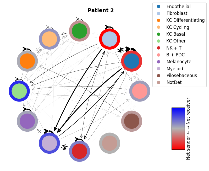
mmcci.pl.network_plot(patient_2_integrated.assays['filtered']['overall'], node_colors=colors, title='Patient 2')
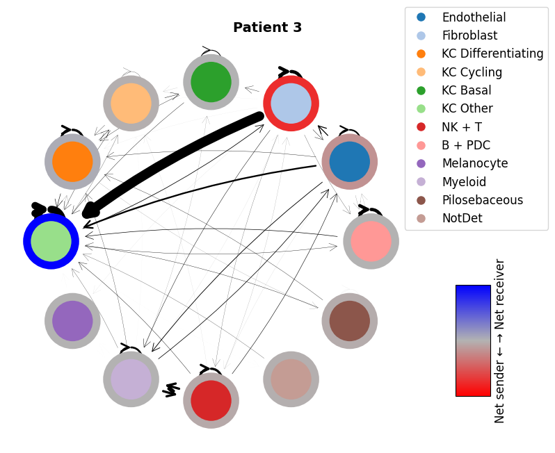
mmcci.pl.network_plot(patient_3_integrated.assays['filtered']['overall'], node_colors=colors, title='Patient 3')
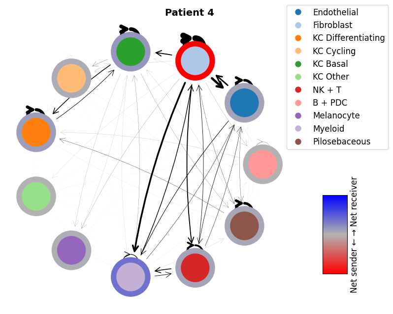
mmcci.pl.network_plot(patient_4_integrated.assays['filtered']['overall'], node_colors=colors, title='Patient 4')

Analysis

Here we will have a look deeper into some specific interactions relevant to the disease

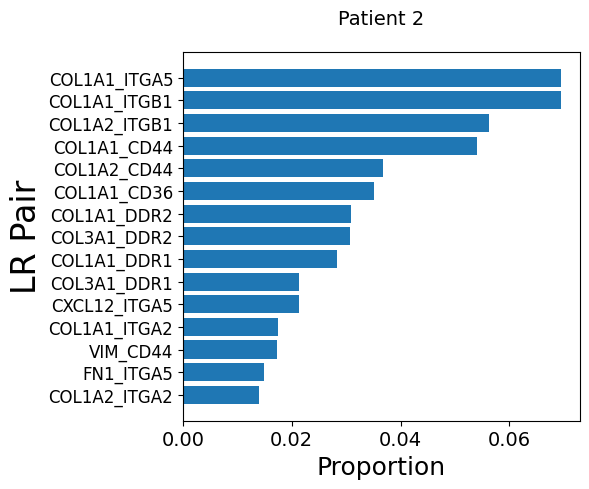
Get LR pairs and pathways from fibroblasts to endothelial cells for each patient

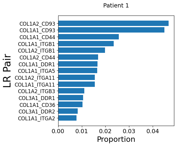
mmcci.pl.lrs_per_celltype(patient_1_integrated, "Fibroblast", "Endothelial", title='Patient 1')
mmcci.pl.lrs_per_celltype(patient_2_integrated, "Fibroblast", "Endothelial", title='Patient 2')
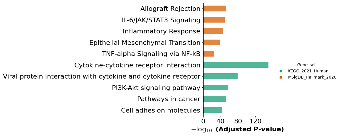
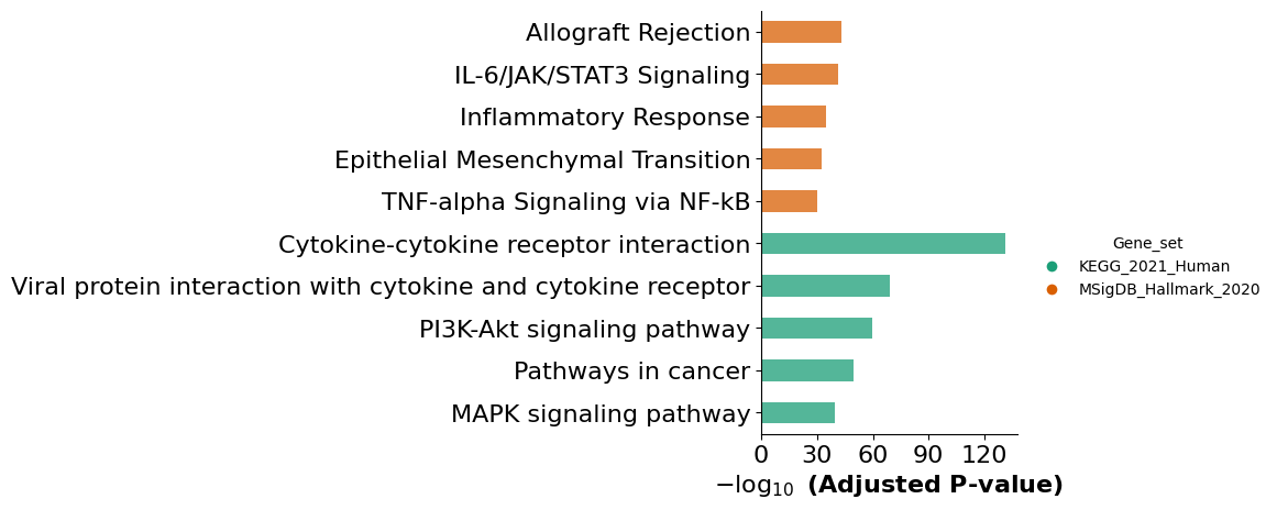
mmcci.an.run_gsea(patient_1_integrated, lrs=patient_1_integrated.get_lr_proportions("Fibroblast", "Endothelial", assay='filtered'), return_results=False)
mmcci.an.run_gsea(patient_2_integrated, lrs=patient_2_integrated.get_lr_proportions("Fibroblast", "Endothelial", assay='filtered'), return_results=False)

results = mmcci.an.run_gsea(integrated, assay="filtered", gene_sets=["KEGG_2021_Human", "MSigDB_Hallmark_2020"], show_barplot=False)

integrated = mmcci.an.pathway_subset(integrated, assay="filtered", gsea_results=results, terms=["Epithelial Mesenchymal Transition"], strict=True, assay_name="EMT")
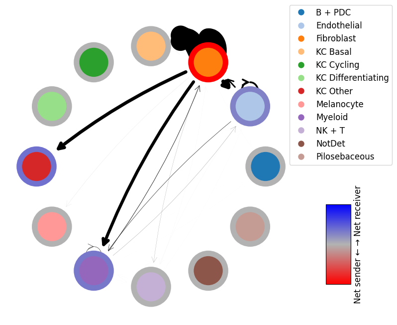
mmcci.pl.network_plot(integrated.assays["EMT"]["overall"], remove_unconnected=False)

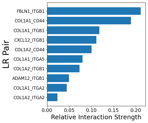
mmcci.pl.lr_barplot(integrated, assay="EMT", n=10)

Number of interactions in EMT: 35